Oreoscoptes Distribution in BC

Introduction

Wildlife preservation in British Columbia (BC) is an important topic to address. Having diverse wildlife could lead to a number of benefits, such as thriving ecosystems (e.g. diverse species lead to more balanced and resilient ecosystems; Ferrero & Troìa, 2021), or economic benefits (e.g. BC’s natural environment is a factor that attracts many tourists yearly, and having wildlife diversity is important to maintaining the health of BC’s nature).

One wildlife species that may be important to conserve is the Sage Thrasher (oreoscoptes montanus). In BC, the population of the sage thrasher has been in decline, due to a number of factors, such as climate change or human activity (e.g. urbanization or agricultural expansion). For example, estimates have shown up to a 50% decline in sage thrasher population over the past century. Furthermore, the sage thrasher has also been designated as endangered by BC Ministry of Environment, and is generally considered a rare bird species in Canada (British Columbia Ministry of Environment and Climate Change Strategy, 2019).

As such, the current investigation aims to investigate ways to preserve the conversation of sage thrashers in BC by conducting a spatial statistical analysis of the species in BC. In particular, we focus on three questions. First, we examine the spatial distribution of sage thrashers in BC (e.g., understanding where sage thrashers are situated could help understanding of where to avoid human expansion). Second, we examine the environmental covariates that are linked to the population of sage thrashers (e.g., understanding factors that promote or hinder sage thrasher population could lead to insights on how to cultivate this species). Third, we build regression models that use covariates to predict the geographical intensity of sage thrashers (e.g., this may lead to insights of geographical areas where environmental conditions are suitable to cultivate new populations of sage thrashers).

Methods

Data Description: Briefly describe the data and what variables are included.

To investigate our research question of how we could preserve sage thrasher population, we downloaded data on sage thrashers from the Global Biodiversity Information Factility (GBIF, 2023). This dataset contains information about where sage thrashers have been sighted (e.g., country, coordinates), of which contains 850 samples in British Columbia. To examine how covariates are related to sage thrasher populations, we obtained data on BC environmental covariates provided by Michael Noonan (Noonan, 2022). This dataset contains measurements on four environmental covariates (that is, elevation, distance to water, forest, and HFI) across spatial areas in BC (ranging from one million to 7 million measurements).

Detailed Analytical Workflow

Our statistical analysis process involved the following four steps: 1) Preparing the data for analysis, such as obtaining and wrangling data, 2) Conducting spatial distributional analysis of sage thrashers, 3) Linking environmental covariates to sage thrashers, 4) Creating regression models for sage thrashers.

1) Data Preparation

1.1) Load all packages we need. Please refer to Statistical Packages.

1.2) Data processing:

• Load Oreoscoptes data by df <- read.csv("BC_data.csv", stringsAsFactors = FALSE).

• Generate a dataframe coord with longitude and latitude in BC_data by

  coord <- df[,c('decimalLatitude','decimalLongitude')].

• Clean the data by removing the observations with NA, coord <- na.omit(coord).

• Visualize the data plot(coord$decimalLatitude, coord$decimalLongitude).

• By using the coordinates function to create a new object with the spatial coordinates and then setting its CRS using proj4string, we can ensure that our spatial analyses are performed correctly, and we can compare our results with other analyses that use the same CRS.

• Load the covariates data by load("BC_Covariates.Rda").

• Define the observation area, window, by win = as.owin(DATA$Window)

• create ppp object with coordination and the window by

2) Spatial Analysis of Sage Thrashers

2.1) Spatial Analysis of Sage Thrashers

• Check the spread of the bird plot(ppp_birds)

• Check homogeneity, perform quardratic test.

• Hot spot analysis to identify areas of elevated intensity by

3) Linking Environmental Covariates to Sage Thrashers

3.1) Linking Environmental Covariates to Sage Thrashers

• Identify the class of each potential covariate by sapply(DATA, class)

• Visualise each potential covariate using methods appropriate to each object class.

• Check relationships between potential covariates via kernel estimation by rhohat

  4) Regression Models for Sage Thrashers

  4.1) Building the Model

  • Scale the covariates by their mean and variance

  • Establish formula1:

  • Fit the model with formula1 by fit1 <- ppm(formula1, data = DATA).

  • Because the model did not converge, we simplified our formula by excluding I(Elevation_scaled^2).

  • Fit the model with formula2 by fit2 <- ppm(formula2, data = DATA).

  • Test the statistical significance of coefficients by looking at the Ztest fromfit2 table.

  • Identify the formula with coefficients co <- coef(fit2)

  • Model visualisation

  • Compute the intensity of a fitted point process model as a function of one of its covariates

  4.2) Validating Regression Model

  • Quardratic Counting by quadrat.test(fit2, nx = 2, ny = 4)

  • Create partial residual plots.

  4.3) Building Advanced GAM Model

  • Build GAM model with 3 degrees of freedom for both covariates.

  • Plot partial residuals for both covariates.

  • Visualize the gam model.

  Packages Employed.

  1. sp: A package providing classes and methods for spatial data: points, lines, polygons and grids
  2. dplyr: A Grammar of data manipulation.
  3. sf: Create sf object.
  4. spatstat: Its main focus is the analysis of spatial patterns of points in two-dimensional space.
  5. maptools: Translate and disguise coordinate placing in the real world.
  6. rgdal: Provide functions for geospatial data.
  7. splines: Create cubic functions.

  Results

2) Spatial Analysis of Sage Thrashers

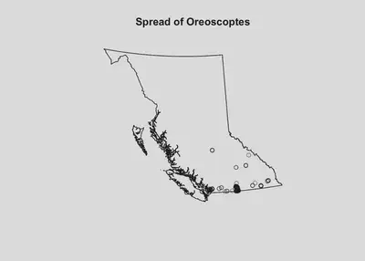
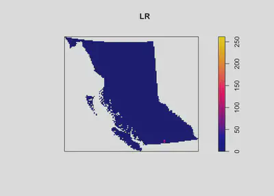
By looking at Figure 1, we can see that the data is not homogeneous dataset as the birds tend to be clustered in south areas of BC, whereas others have no birds at all, and we conduct a quardratic test to support the inhomogeneous assumption (small p-value). Figure 2 illustrates the hotspot is Osoyoos of the dataset.

3) Linking Environmental Covariates to Sage Thrashers

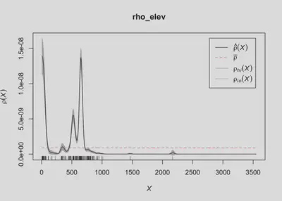
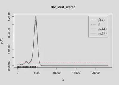
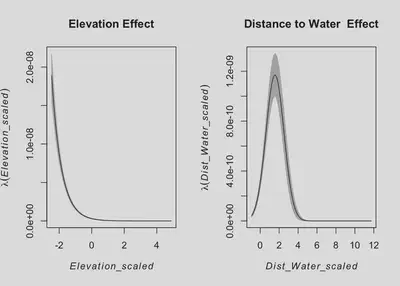
There are four potential covariates in BC_Covariates.Rda, Elevation, Forest, HFI, and Dist_Water. It’s hard to tell the relationship between them and intensity, so we used kernel estimation to detect it. Figure 3 shows that there seem to be two clusters: one group lives near the 0 elevation, and another group lives at around 500m, and there is a non-linear relationship between elevation and bird intensity. The narrow band in Figure 4 describes a specific preference for habitats in terms of the distance to water, and a non-linear relationship between it and bird intensity as well (with one group clustered at 3-5km away from water sources). We exclude Forest and HFI here because of wider bandwidths.

4) Regression Models for Sage Thrashers

4.1) Building the Model 4.2) Validating the Model

After deciding to use Elevation and Dist_Water to be candidate of covariates with quardratic effect, we scaled both variables to prevent disproportional impact on bird intesity to build the regression model with formula1: ppp_birds ~ Elevation_scaled + I(Elevation_scaled^2) + Dist_Water_scaled + I(Dist_Water_scaled^2).

However, when we tried to fit first model, it failed to converge. Hence, we simplified our formula to formula2: ppp_birds ~ Elevation_scaled + Dist_Water_scaled + I(Dist_Water_scaled^2) by excluding the I(Elevation_scaled^2) and built a second model. By the Ztest from the model, we can say that all the coefficients are statistically significant. It suggested that the intensity can be estimated by the following function:

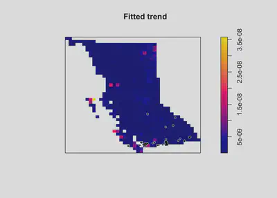
$\lambda(u)$ = exp(r co[1] + r co[2] Elevation_scaled + r co[3] Dist_Water_scaled + r co[4] * I(Dist_Water_scaled^2))

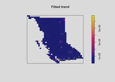
Figure 5 shows that with these two covariates, the model predicts two novel areas: Vancouver Island and Graham Island as suitable areas to cultivate new sage thrasher species.

However, as will be elaborated upon in the discussion section, these suggestions should be interpreted with caution becauase it is possible that our model may not be making these predictions accurately, as we can see that our model performance may not be accurate, as there are no true observations (observation black dots) model’s predicted areas (yellow).

To see how individual coefficients affect the intensity, please follow figure 6. It indicates that Elevation has negative marginal effect before it reaches its mean value (Elevation_scaled > 0). On the other hand, Distance_Water has greatest marginal effect at 2 standard deviation away from its mean value and then the effect goes down.

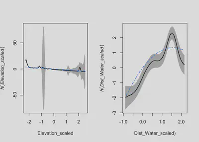
Though by Figure 5 we can see that the model did not fit well to our dataset, we performed a quadrat test to be more sure about it. The small p-value shows that there’s a significant deviation from our model’s predictions. Hence, we used the residual plot to see how to enhance it. From Figure 7 we can see that the quadratic terms are not capturing the patterns in our data particularly well. As an improvement, we could try adding higher-order polynomials, but polynomials can be unstable. In this situation, we tried to switch from a linear modelling framework, to an additive modelling framework (i.e., GAMs).

4.3) Advanced GAM Model

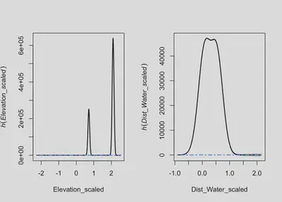
With a gam with degree of freedom 3 for both covariate, Figure 8 shows that the spline term still could not capture the trends. And Figure 9 illustrates that the model still not fit the dataset.

Discussion

The present investigation aimed to examine how sage thrasher population could be preserved in BC by focusing on three questions. First, we investigated the spatial distribution of sage thrashers in BC. Our analysis showed that sage thrashers are significantly disproportionately located in the southern areas of BC. Second, we investigated covariates that are linked to sage thrasher populations. Our analysis found that the covariates of elevational height (i.e., low elevations of 0 and 500 meters) and distance to water (i.e. proximities of 3000-5000 meters to water) are predictors that are positively linked to sage thrasher intensity in BC. Third, our analysis investigated regression models to predict areas in which sage thrasher populations would thrive. Our regression models predicted that areas along the western coastlines of BC (e.g. Graham island, Vancouver island) are linked to high intensity of sage thrasher populations.

The findings from the current analysis provide insights into ways that sage thrasher populations could be preserved in BC. First, the analysis suggests that areas in southern BC are primarily where sage thrashers are located (e.g., urbanization of these areas should be discouraged). Second, the analysis suggests that, to cultivate sage thrashers, it would beneficial to build their habitats around 3 to 5 kilometres away from water sources, in elevations of 0 or 500 meters. Third, our analysis predicts that, based off of covariates that predict thriving sage thrasher populations, two new areas that could be suitable to cultivate new populations of sage thrashers are Vancouver Island and Graham islands.

Although the current analysis provides several insights into sage thrasher conservation, there are also a number of limitations. One limitation relates to the methodology of the study. For example, given the rarity of sage thrashers in BC, there was only a small sample size of sage thrashers (i.e. around 800 sage thrashers) to base our analysis upon, which could limit the statistical accuracy of our findings (e.g., higher likelihood of statistical errors due to small samples). Second, the current analysis was only able to obtain a small number of environmental covariates to link sage thrasher populations to, which may hinder the ability to understand true and more important predictors that may allow sage thrasher populations to thrive (e.g., weather). As such, future studies should aim to incorporate higher sample sizes of sage thrashers, and greater numbers of environmental covariates to link to sage thrashers.

Another limitation relates to the statistical validity of our findings. For example, although our regression models predicted suitable areas for sage thrasher populations, diagnostics show that our basic and advanced GAM models may not fully capture trends in data effectively. Future studies should xxx.

References

British Columbia Ministry of Environment and Climate Change Strategy. (2019). Sage Thrasher. Government of British Columbia. https://www2.gov.bc.ca/assets/gov/environment/plants-animals-and-ecosystems/species-ecosystems-at-risk/brochures/sage_thrasher.pdf

Ferrero, P., & Troìa, A. (2021). The Role of Biodiversity in Ecosystem Resilience. Sustainability, 13(14), 7681. https://doi.org/10.3390/su13147681

GBIF.org. (2023). Ixodes ricinus Linnaeus, 1758. GBIF Occurrence Download. https://www.gbif.org/species/2494973

Noonan, M. (2022, January 15). Data-589 [GitHub repository]. GitHub. https://github.com/ubco-mds-2022/Data-589